MATLAB Cluster Based Routing Protocol Code: Implementation, Architecture, and Simulation Guide
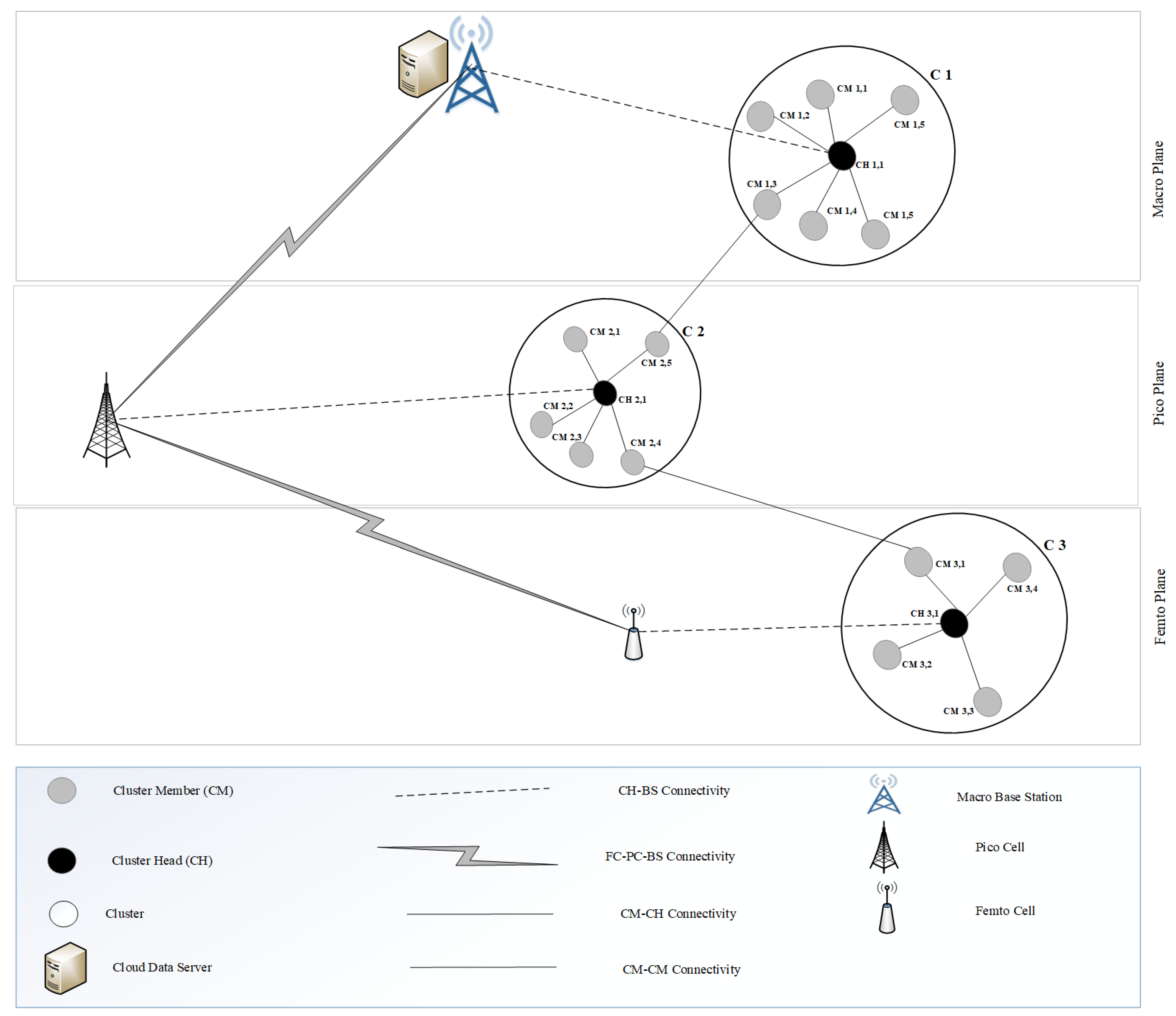
Implementing a MATLAB cluster based routing protocol code allows researchers and network engineers to simulate energy-efficient wireless sensor networks, optimize data aggregation, and evaluate network lifetime under various algorithmic constraints.
Cluster-based routing protocols in Wireless Sensor Networks (WSNs) partition the network into distinct groups of nodes, known as clusters. Within each cluster, a designated node—frequently referred to as the Cluster Head (CH)—aggregates local sensing data and transmits it across a longer distance to a central base station (sink). This hierarchical architecture significantly reduces energy consumption compared to flat multi-hop or direct transmission models.
MATLAB provides a robust computational environment and object-oriented programming framework to model these discrete-event or round-based protocols, visualize node energy depletion, and benchmark performance metrics such as throughput, packet delivery ratio, and dead-node timelines.
Understanding Cluster-Based Routing Foundations in WSNs
Wireless sensor networks operate under strict resource constraints, primarily driven by battery-powered nodes that are often deployed in hostile or inaccessible environments. Because node replacement is frequently impractical, energy conservation stands as the absolute priority in protocol design. Flat routing topologies, where every node relays traffic for its neighbors, often cause premature energy depletion near the base station—a phenomenon known as the energy hole problem.
The Role of Clustering Architectures
Clustering divides the network topology into localized substructures, transforming a massive global routing problem into manageable local interactions.
- Intra-Cluster Communication: Sensor nodes within a specific geographic radius transmit their sensory data exclusively to their local Cluster Head. This short-range communication minimizes transmission power levels.
- Data Aggregation and Fusion: The Cluster Head processes raw packets from multiple members, eliminating redundancy, compressing the payload, and forwarding a unified data packet.
- Inter-Cluster Communication: Cluster Heads communicate either directly with the base station or through multi-hop paths formed by other CHs, distributing the heavy routing burden across rotating nodes.
Protocol Lifecycle: Setup and Steady-State Phases
Simulating these dynamics in MATLAB requires structuring the code into repeating operational cycles, or rounds. Each round typically comprises two primary phases:
- Setup Phase: Nodes evaluate their residual energy, probabilistic thresholds, or proximity metrics to elect themselves as Cluster Heads or associate with the nearest available CH.
- Steady-State Phase: Data transmission occurs. Nodes wake up, sample the environment, send data to their CH during allocated Time Division Multiple Access (TDMA) slots, and return to sleep mode to conserve power.
Core Components of MATLAB Cluster-Based Routing Implementation
Developing or executing a cluster-based routing protocol script in MATLAB requires several structural blocks. A well-architected simulation framework separates network initialization, physical channel modeling, energy depletion tracking, and performance logging into modular scripts or classes.
1. Network Initialization and Node Deployment
The simulation begins by defining spatial boundaries (e.g., a $100\text{ m} \times 100\text{ m}$ square area) and scattering a defined number of nodes ($N$) either randomly using uniform distributions or deterministically.
% Basic parameters initialization snippet field.x = 100; field.y = 100; sink.x = 50; sink.y = 175; % Base station located outside the sensor field n = 100; % Total number of nodes
Each node is typically instantiated as a structure or a handle class containing properties such as coordinates (x, y), current energy (E), role (type where $0=$ normal node, $1=$ cluster head, $-1=$ dead), distance to the sink, and cluster identification number (clusterID).
2. Energy and Radio Propagation Models
To accurately reflect physical realities, the MATLAB code must implement a standard radio energy dissipation model. The energy consumed to transmit an $L$-bit packet over a distance $d$ is calculated based on whether the distance exceeds a threshold $d_0$:
Free-Space Model ($d < d_0$): $$E_{tx}(L, d) = L \cdot E_{elec} + L \cdot \varepsilon_{fs} \cdot d^2$$
Multipath Fading Model ($d \ge d_0$): $$E_{tx}(L, d) = L \cdot E_{elec} + L \cdot \varepsilon_{mp} \cdot d^4$$
The energy consumed to receive that same $L$-bit packet is: $$E_{rx}(L) = L \cdot E_{elec}$$
Where $E_{elec}$ represents the electronics energy, while $\varepsilon_{fs}$ and $\varepsilon_{mp}$ are amplifier parameters dependent on the transceiver circuitry.
Popular Protocols Modeled in MATLAB
Various foundational and contemporary protocols serve as benchmarks for custom MATLAB implementations. Understanding their unique mechanisms helps ensure the underlying code accurately reflects the intended routing logic.
| Protocol Name | Core Mechanism | Selection Metric | Primary Advantage | Typical MATLAB Modeling Focus |
|---|---|---|---|---|
| LEACH | Randomized rotation of CHs | Probabilistic threshold based on rounds | Distributed, simple, extends network lifetime over direct routing | Evaluating random energy decay and first node death rounds. |
| HEED | Hybrid energy-efficient distributed clustering | Residual energy and node degree/cost | Well-distributed CHs, handles dense deployments effectively | Analyzing iterative neighbor discovery and cost calculations. |
| SEP | Stable Election Protocol for heterogeneous networks | Weighted probabilities based on initial energy levels | Accounts for advanced and normal nodes, prolongs stability period | Modeling multi-level energy distribution arrays. |
| TEEN | Threshold-sensitive Energy Efficient sensor Network | Reactive thresholding for time-critical applications | Reduces transmissions by reporting only on significant metric changes | Implementing reactive event-driven state machines. |
Step-by-Step Breakdown of a Typical MATLAB Routing Script
Writing a complete simulation script involves orchestrating initialization, round loops, and post-processing analytics. The following architectural outline details how these elements connect within the MATLAB workspace.
Step-by-Step Execution Flow
- Parameter Setup: Define global constants including packet size, initial energy ($E_0$), transmitter/receiver electronics dissipation, amplifier constants, and maximum number of simulation rounds.
- Node Array Generation: Populate matrices or object arrays with random spatial coordinates and assign baseline energy values.
- Round Iteration Loop (
for r = 1:max_rounds):- Check for network depletion (break loop if all nodes are dead).
- Execute cluster head selection algorithms (e.g., evaluating threshold formulas for probabilistic protocols).
- Broadcast CH announcements and execute node-to-CH association based on Received Signal Strength Indicator (RSSI) or Euclidean distance.
- Allocate TDMA schedules for intra-cluster communication.
- Calculate energy consumed for data sensing, transmission, aggregation, and reception for every active node.
- Update residual energy levels and flag dead nodes ($E \le 0$).
- Data Logging and Visualization: Record metrics such as live nodes per round, total data packets received at the base station, and average residual energy. Update MATLAB figure windows dynamically to display cluster formations.
Example Code Structure: Implementing LEACH-Style Clustering
Below is an illustrative structural template representing core sections of a MATLAB script for a round-based cluster routing protocol. This demonstrates how node loops and energy updates are typically handled.
% Initialization clear; clc; numOfNodes = 100; P = 0.1; % Desired percentage of cluster heads Eo = 0.5; % Initial energy in Joules Eelec = 50*10^(-9); ETX = 50*10^(-9); ERX = 50*10^(-9); Efs = 10*10^(-12); Emp = 0.0013*10^(-12); EDA = 5*10^(-9); % Data aggregation energy packetLength = 4000; % bits maxRounds = 1000; % Create Node Structure for i = 1:numOfNodes node(i).x = rand * 100; node(i).y = rand * 100; node(i).energy = Eo; node(i.type) = 'N'; % N: Normal, C: Cluster Head, D: Dead node(i).G = 0; % Round eligibility counter end % Simulation Rounds Loop for r = 1:maxRounds numDeadNodes = 0; % Check energy status for i = 1:numOfNodes if node(i).energy <= 0 node(i).type = 'D'; numDeadNodes = numDeadNodes + 1; end end % Cluster Head Election Phase (LEACH style threshold) for i = 1:numOfNodes if node(i).type ~= 'D' if node(i).G <= 0 temp_rand = rand; threshold = P / (1 - P * mod(r, round(1/P))); if temp_rand < threshold node(i).type = 'C'; node(i).G = round(1/P); end end end end % Association and Transmission Phase omitted for brevity... % Energy subtraction calculations occur here based on distance to CH/Sink. end
Verifying and Troubleshooting MATLAB Routing Simulations
When executing complex routing scripts, common numerical or logical errors can distort simulation results. Proper verification ensures the reliability of published or academic findings.
Common Implementation Pitfalls
- Negative Energy States: Failing to check node energy before subtraction can lead to negative energy values, artificially inflating network lifetime metrics. Always clamp energy floors at zero.
- Orphaned Nodes: If a cluster head dies mid-round or if deployment densities leave isolated nodes without a reachable CH, transmission calculations will fail or produce infinite loops. Implement fallback direct-transmission routines for unassigned nodes.
- Vectorization vs. For-Loops: While MATLAB excels at vectorized matrix operations, complex state-dependent routing protocols often require explicit
forloops to handle dynamic neighbor discovery and sequential packet forwarding. Balance performance optimization with code readability.
Performance Evaluation Metrics
To validate your MATLAB code, compute and plot the following standard metrics:
- Stability Period: The number of rounds elapsed until the very first node exhausts its energy.
- Network Lifetime: Measured typically by FND (First Node Dead), HND (Half Nodes Dead), and LND (Last Node Dead).
- Throughput: The cumulative number of data packets successfully delivered to the sink node across all simulation rounds.
Frequently Asked Questions
How do I incorporate node mobility into a MATLAB cluster-based routing code?
Node mobility requires updating spatial coordinates (x, y) at the beginning of every round or frame using a mobility model such as the Random Waypoint Model. When nodes move, cluster formations and inter-node distances must be recalculated dynamically, increasing computational overhead within the MATLAB environment.
Why is my MATLAB code running extremely slowly during large simulations?
Slow execution is frequently caused by nested for loops checking pairwise Euclidean distances across large node arrays ($N > 500$). To improve performance, replace explicit loops with vectorized matrix distance calculations using functions like pdist2 and pre-allocate memory for tracking arrays prior to entering the round loop.
How can I modify existing LEACH code to simulate heterogeneous energy nodes?
Heterogeneous protocols like SEP or DEEP require assigning different initial energy levels to nodes during the initialization phase (e.g., advanced nodes start with $1.5 \times E_0$). The CH election threshold formula must then be weighted relative to the node's initial energy share compared to normal nodes.
Can I interface my MATLAB routing code with network simulators like NS-2 or NS-3?
Yes. While MATLAB handles mathematical modeling and algorithmic optimization efficiently, you can export node deployment files and routing schedules into text formats readable by network simulators like NS-2 or NS-3 for packet-level validation under realistic MAC layer protocols.
Conclusion and Next Actions
Implementing a MATLAB cluster based routing protocol code requires a systematic approach to network topology generation, energy consumption modeling, and iterative round execution. By structuring scripts cleanly around modular setup, cluster head election, data transmission, and logging phases, researchers can accurately evaluate protocol performance and energy efficiency. To proceed further, begin by executing a baseline LEACH simulation, verify energy depletion curves against established literature, and incrementally introduce advanced parameters like node heterogeneity or multi-hop inter-cluster routing.
Image Gallery
Select an image to open it in a new tab.
