How to Program the IEEE 14 Bus System in MATLAB for Power Flow Analysis

Implementing the IEEE 14 bus test system in MATLAB allows electrical engineering students, researchers, and power systems professionals to model a standard transmission network, perform power flow calculations, and analyze steady-state grid behavior under various operational constraints.
Introduction to the IEEE 14 Bus Test System and MATLAB
The IEEE 14 bus system represents a portion of the American Electric Power system as of February 1962. It is widely used in power systems research as a standard benchmark network for testing power flow algorithms, optimal power flow (OPF), economic dispatch, and contingency analysis. When researchers refer to programming this system in MATLAB, they typically mean creating a structured numerical model of its buses, transmission lines, transformers, and loads, and then executing iterative computational methods—such as the Newton-Raphson, Fast Decoupled, or Gauss-Seidel algorithms—to solve the non-linear power flow equations.
MATLAB provides a robust matrix-manipulation environment well-suited for handling the admittance matrix (Y-bus) and solving algebraic equations. While commercial or open-source toolboxes like MATPOWER automate these steps, writing custom scripts to program the system from scratch provides deep insight into the underlying mathematics of electrical power systems. This guide explores the structure of the IEEE 14 bus network, the necessary MATLAB data formats, core programming steps, and validation techniques required to run successful simulations in 2026.
Understanding the IEEE 14 Bus System Architecture
Before writing any code, you must understand the physical and topological composition of the IEEE 14 bus network. A standard test case configuration consists of specific components that dictate how power flows through the transmission grid.
The network comprises 14 nodes, or buses, categorized into different types based on their control variables. It also contains multiple transmission lines, transformers with specific tap settings, and shunt susceptance compensation devices. Understanding these components ensures your MATLAB data matrices accurately reflect physical reality.
Bus Classifications and Data Fields
In power flow programming, buses are generally classified into three operational types:
- Swing Bus (Slack Bus): Bus 1 serves as the slack bus. It absorbs or generates the active and reactive power imbalance required to match total system losses and fixes the voltage magnitude and phase angle ($\theta = 0^\circ$).
- Generator Buses (PV Buses): Buses 2, 3, 6, and 8 are equipped with generators. For these nodes, the active power generation ($P_G$) and voltage magnitude ($|V|$) are specified, while the reactive power ($Q$) and phase angle are calculated.
- Load Buses (PQ Buses): The remaining nodes (Buses 4, 5, and 7 through 14) are pure load buses where active power demand ($P_D$) and reactive power demand ($Q_D$) are known, and voltage magnitude and phase angles are unknown.
Branch and Transformer Characteristics
The branch data specifies the connections between buses. The IEEE 14 bus system includes transmission lines and regulating transformers. Each branch entry requires parameters such as:
- From Bus and To Bus indices.
- Resistance ($R$) and Reactance ($X$) in per-unit (p.u.).
- Total line charging susceptance ($B/2$) in per-unit.
- Transformer tap ratios and phase shift angles (where applicable).
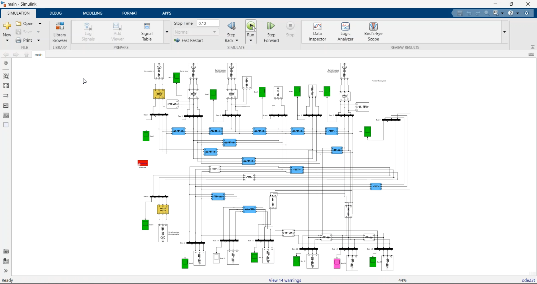
Prerequisites and Software Environment Setup
Setting up your workspace correctly prevents common matrix dimension mismatches and numerical convergence failures during execution.
You need a working installation of MATLAB. While basic base MATLAB is sufficient for writing custom Newton-Raphson solvers, having the Power System Toolbox or utilizing established packages like MATPOWER can simplify data structure management. However, writing custom scripts requires familiarity with core MATLAB syntax, sparse matrices, and iterative loop controls.
Required Mathematical Formulation
The foundation of any power flow program is the nodal admittance matrix, commonly known as the Y-bus matrix. The Y-bus matrix relates nodal injected currents to nodal voltages:
$$I = Y_{bus} V$$
For a system with $N$ buses, $Y_{bus}$ is an $N \times N$ complex matrix. Off-diagonal elements represent the negative admittance of the branches connecting the respective buses, while diagonal elements represent the sum of all admittances connected to that specific bus, including line charging and shunt elements.
Step-by-Step Guide to Programming the System in MATLAB
Implementing the power flow program involves structuring input data, building the Y-bus matrix, initializing variables, and running an iterative solver until convergence is achieved. Below is a structured technical workflow.
Step 1: Define the Input Data Structures
Create structured arrays or matrices for your bus data and branch data. Following standard formats (similar to MATPOWER conventions), your matrices should contain columns for indices, types, loads, generation, voltage initial guesses, base voltage, and network limits.
% Example structure concept for Bus Data % Col 1: Bus Number % Col 2: Bus Type (1=PQ, 2=PV, 3=Slack) % Col 3: Pd (Active load, MW) % Col 4: Qd (Reactive load, MVAR) % Col 5: Gs (Shunt conductance, MW) % Col 6: Bs (Shunt susceptance, MVAR) % Col 7: Area number % Col 8: Voltage magnitude initial guess (p.u.) % Col 9: Voltage angle initial guess (degrees)
Step 2: Construct the Y-Bus Matrix
Write a MATLAB script that loops through the branch data to assemble the $14 \times 14$ complex admittance matrix. Utilize sparse matrix functions (sparse()) to optimize memory if scaling to larger systems, though a dense matrix is manageable for a 14-bus configuration.
function Ybus = makeYbus(baseMVA, bus, branch) nb = size(bus, 1); nl = size(branch, 1); % Extract parameters fbus = branch(:, 1); tbus = branch(:, 2); r = branch(:, 3); x = branch(:, 4); bc = branch(:, 5); tap = branch(:, 6); tap(tap == 0) = 1.0; % Default tap ratio z = r + 1j * x; y = 1 ./ z; bc = 1j * bc / 2; Ybus = sparse(nb, nb); % Add branch admittances for k = 1:nl i = fbus(k); j = tbus(k); y_branch = y(k) / tap(k); y_sh_f = y(k) * (1 - tap(k)) / (tap(k)^2); y_sh_t = y(k) * (tap(k) - 1) / tap(k); Ybus(i, i) = Ybus(i, i) + y(k) / (tap(k)^2) + bc(k); Ybus(j, j) = Ybus(j, j) + y(k) + bc(k); Ybus(i, j) = Ybus(i, j) - y_branch; Ybus(j, i) = Ybus(j, i) - y_branch; end % Add shunt admittances from bus data gs = bus(:, 5); bs = bus(:, 6); Ybus = Ybus + sparse(1:nb, 1:nb, gs + 1j*bs, nb, nb); end
Step 3: Implement the Newton-Raphson Solver Loop
The Newton-Raphson method is the industry standard for solving power flow equations due to its quadratic convergence characteristics. The algorithm calculates power mismatches ($\Delta P$ and $\Delta Q$), builds the Jacobian matrix, solves for corrections to voltage magnitudes and angles, and updates the state variables iteratively.
% Core iterative update structure in Newton-Raphson tolerance = 1e-5; max_iterations = 100; converged = false; for iter = 1:max_iterations % 1. Calculate calculated P and Q at each bus % 2. Compute mismatch vectors dP and dQ % 3. Check convergence criteria (max(abs([dP; dQ])) < tolerance) % 4. Build Jacobian matrix [J1 J2; J3 J4] % 5. Solve linear system: [dTheta; dV] = inv(J) * [dP; dQ] % 6. Update voltage angles and magnitudes end
Comparison of Power Flow Solution Methods in MATLAB
When programming power flow models, developers can choose among several numerical algorithms. Each method has distinct trade-offs regarding computational speed, memory usage, and convergence reliability.
| Algorithm | Convergence Speed | Memory Requirements | Robustness on Ill-Conditioned Systems | Best Used For |
|---|---|---|---|---|
| Newton-Raphson | Very Fast (Quadratic) | Moderate | High | Standard transmission networks, highly accurate studies |
| Fast Decoupled | Fast per iteration | Low | Moderate | Large-scale systems where real/reactive power coupling is weak |
| Gauss-Seidel | Slow (Linear) | Low | Low | Educational demonstrations, small radial distribution networks |
Common Programming Mistakes and Troubleshooting
Developing power flow code from scratch frequently introduces subtle bugs. Reviewing common pitfalls helps streamline debugging.
Per-Unit System Inconsistencies
Ensure all network parameters (impedances, loads, generations) are converted to a common system base (typically 100 MVA). Mixing physical units (ohms or megawatts) directly into admittance matrices without per-unit normalization leads to incorrect voltage profiles and divergence.
Jacobian Singularity and Matrix Ill-Conditioning
If your Newton-Raphson solver fails to converge or throws a matrix singularity error, inspect your Jacobian matrix. Common causes include:
- Failing to properly isolate the slack bus angle and voltage magnitude from the Jacobian matrix rows/columns.
- Excessive reactive power limits violations on PV buses without proper switching of bus types.
- Incorrect branch tap ratios resulting in division by zero or extremely high admittances.
Verification of Results
To verify that your programmed IEEE 14 bus MATLAB script functions correctly, compare your output values against established benchmarks. In a standard IEEE 14 bus solution (with a 100 MVA base), the voltage magnitude at Bus 1 (slack) should remain fixed at 1.060 p.u. with an angle of $0^\circ$. Load bus voltages typically range between 1.00 p.u. and 1.06 p.u., and total system active power losses should hover around 13.3 MW under base case loading conditions, depending on precise line parameter definitions.
Frequently Asked Questions
Can I use built-in MATLAB toolboxes to run the IEEE 14 bus system?
Yes. If you have the MATLAB Power System Simulation Toolbox or download the open-source MATPOWER package, the IEEE 14 bus test case is included natively as case14.m. You can load and solve it instantly using commands like runpf('case14').
Why does my Newton-Raphson program diverge after a few iterations?
Divergence usually stems from an incorrect initial flat start voltage guess, an improper Y-bus matrix construction where shunt elements are inverted, or severe reactive power limit violations on generator buses that require manual bus-type switching.
How do I modify line parameters to simulate a contingency?
You can simulate a line outage by locating the specific row in your branch data matrix corresponding to the transmission line and setting its resistance and reactance to extremely high values (or setting its status flag to zero if your code supports status filtering), which effectively removes it from the Y-bus calculation.
Is a flat start mandatory for voltage initialization?
No, but it is standard practice. A flat start initializes all load bus voltage magnitudes to 1.0 p.u. and phase angles to $0^\circ$. For heavily stressed systems, utilizing a warm start based on previous operating points improves convergence speed.
Conclusion and Next Actions
Programming the IEEE 14 bus system in MATLAB bridges theoretical power system analysis with practical computational implementation. By properly organizing bus and branch data, accurately building the Y-bus matrix, and implementing an iterative solver like Newton-Raphson, you establish a powerful platform for advanced grid analysis. To expand your project further, consider integrating optimal power flow (OPF) constraints, incorporating renewable energy intermittency profiles, or testing contingency scenarios under various loading conditions.
Image Gallery
Select an image to open it in a new tab.
