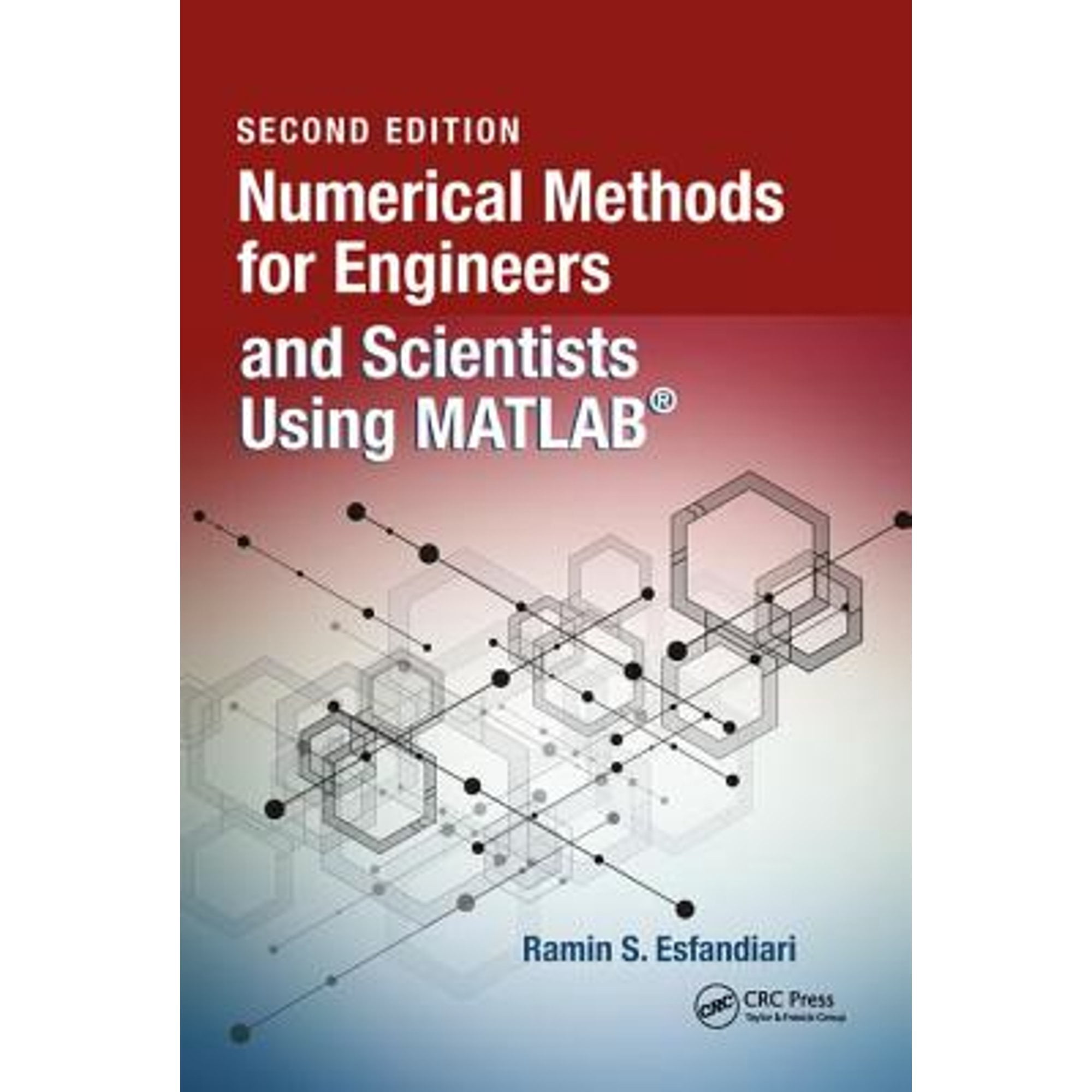
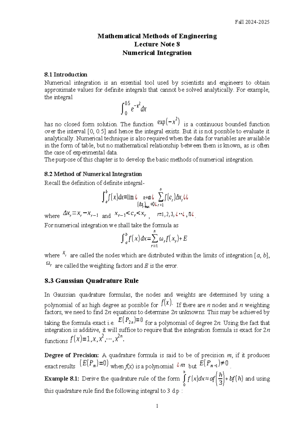
Comprehensive Numerical Methods for Engineers 6th Solution Guide (2026 Edition)
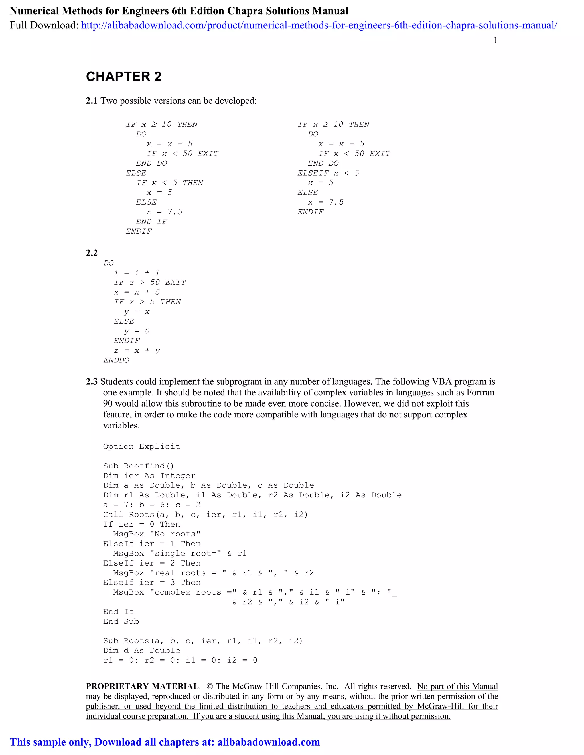
Clarification Note: This technical reference addresses the analytical formulations, algorithmic derivations, and step-by-step verification protocols for problem sets found in the sixth edition of "Numerical Methods for Engineers" by Steven C. Chapra and Raymond P. Canale.
Mastering computational engineering requires bridging pure mathematical theory and applied algorithmic execution. The sixth edition of Chapra and Canale's standard text remains a cornerstone curriculum benchmark worldwide across mechanical, civil, chemical, and aerospace disciplines. While raw answer keys often circulate without context, true engineering competency depends on dissecting error propagation, ensuring convergence stability, and implementing robust solution strategies.
Evaluating these numerical mechanics requires understanding why particular algorithms fail, how round-off errors accumulate in floating-point operations, and how to structure verifiable solutions manually and computationally.
Foundational Mathematical Modules in the 6th Edition Curriculum
The architecture of the sixth edition divides numerical analysis into distinct operational domains. Each domain addresses specific physical behaviors modeled by mathematical operators, ranging from algebraic balance equations to multi-dimensional transport phenomena.
1. Roots of Equations and Bracketing Mechanics
Finding the roots of nonlinear transcendental equations represents the most fundamental task in engineering design, appearing in friction-factor calculations, equation-of-state evaluations, and structural deflection equilibria.
- Bracketing Methods: Bisection and False-Position (Regula Falsi) require two initial guesses that bracket a sign change, satisfying the condition where the product of the function evaluated at the lower and upper bounds is strictly negative. While bisection guarantees convergence with linear speed, false-position utilizes linear interpolation between points to accelerate convergence, though it can stall when dealing with high-order curvature.
- Open Methods: Newton-Raphson and Secant formulations eliminate the requirement for bounds but sacrifice guaranteed stability. Newton-Raphson relies on evaluating the first derivative at the current estimate. It achieves quadratic convergence near simple roots, meaning the number of significant correct digits roughly doubles with each iteration cycle.
2. Linear Algebraic Systems and Matrix Factorization
Engineering systems modeled by coupled discrete nodes—such as truss networks, steady-state thermal distribution grids, and chemical reactor arrays—yield systems of simultaneous linear algebraic equations expressed in matrix notation.
- Direct Elimination Methods: Gauss elimination systematically transforms the coefficient matrix into an upper triangular system via forward elimination, followed by backward substitution. Naive elimination fails under zero-pivot conditions and generates catastrophic truncation errors when diagonal elements are magnitudes smaller than surrounding values. Partial pivoting maintains operational stability by dynamically swapping rows to secure the largest absolute magnitude in the pivot position.
- Matrix Factorization (LU Decomposition): Algorithms like Doolittle, Crout, and Cholesky decompose the coefficient matrix into lower and upper triangular components. This approach significantly reduces computational complexity when solving identical structural matrices subjected to multiple load vectors.
- Iterative Techniques: The Gauss-Seidel and Jacobi methods execute relaxation sweeps across diagonal-dominant systems. Introducing Successive Over-Relaxation (SOR) factors accelerates convergence in large-scale boundary evaluations.
3. Optimization and Extremum Identification
Moving beyond single-variable root finding, engineering design frequently demands locating minimum cost, maximum structural efficiency, or optimal chemical yield. The text covers one-dimensional approaches such as Golden-Section Search and parabolic interpolation, expanding these concepts into multidimensional unconstrained techniques including Gradient Methods, Steepest Ascent, and Newton's multi-variable optimization.
4. Curve Fitting, Regression, and Interpolation
Experimental data collection introduces measurement noise that must be filtered using analytical models.
- Linear and Polynomial Least-Squares Regression: Minimizes the sum of the squares of the residuals between observed data points and the mathematical model, utilizing normal equations to derive coefficients.
- Interpolation Polynomials: Newton’s divided-difference and Lagrange interpolation yield continuous functions that pass precisely through every measured node. For high-density datasets prone to Runge's phenomenon (wild edge oscillations), the text presents cubic splines, which preserve first and second derivative continuity across all intermediate knots.
Algorithmic Comparison Across Core Engineering Modules
Selecting the appropriate numerical method requires balancing execution speed against memory overhead and stability guarantees. The following table provides an operational baseline comparing the primary methodologies covered in the sixth edition.
| Computational Domain | Analytical Method | Convergence Rate | Stability Profile | Core Engineering Applications |
|---|---|---|---|---|
| Root Location | Bisection Method | Linear | Absolute (if bracketed) | Initial guess isolation, robust failsafe checks |
| Root Location | Newton-Raphson | Quadratic | Conditional (diverges at inflections) | Pipeline friction factor, Redlich-Kwong states |
| Linear Systems | LU Decomposition | Exact (Direct) | High (with partial pivoting) | Structural truss analysis, multiple load cases |
| Linear Systems | Gauss-Seidel | Linear | Conditional (requires diagonal dominance) | Finite-difference thermal conduction meshes |
| Curve Fitting | Cubic Spline Interpolation | Non-Iterative | Extremely Stable | Cam profile design, fluid boundary definitions |
| Numerical Integration | Simpson's 1/3 Rule | Fourth-Order Global | High (for smooth functions) | Cross-sectional flow, total structural strain |
| Numerical Integration | Gauss Quadrature | Exponential | High (optimal interior nodes) | Finite element internal energy formulations |
| Differential Equations | 4th-Order Runge-Kutta (RK4) | Fourth-Order Local | High (non-stiff systems) | Transient circuit response, dynamic motion |
| Differential Equations | Crank-Nicolson (PDE) | Second-Order Space/Time | Unconditionally Stable | Transient 1D/2D heat and mass diffusion |
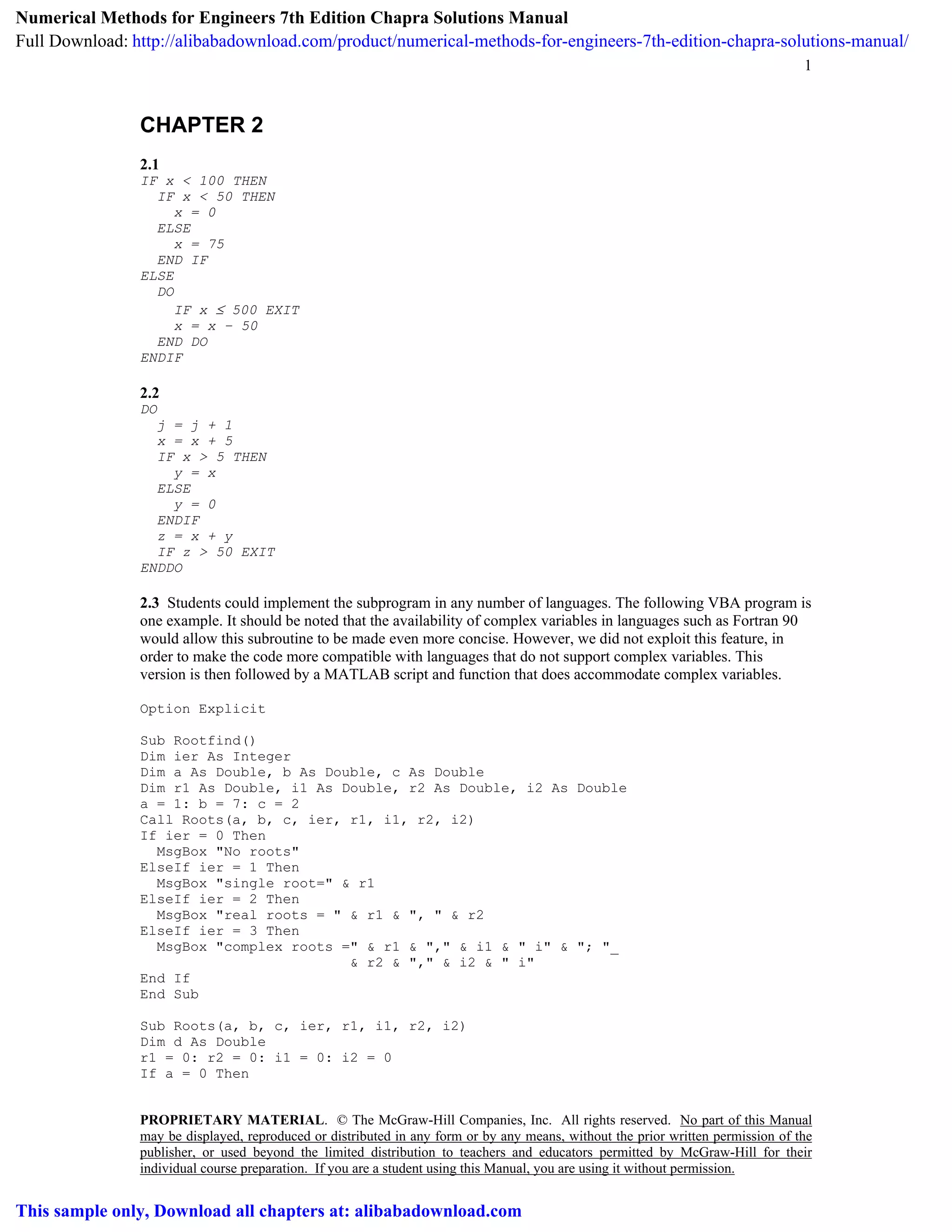
Systematic Problem-Solving Framework for 6th Edition Solutions
Executing homework exercises or design validations from the text requires adhering to a repeatable, four-stage protocol to prevent systemic mathematical drift.
Stage 1: Problem Idealization and Form Transformation
Never apply an iterative method directly to raw physical values without verification.
- Transpose the governing equation into standard root form, f(x) = 0, or matrix form, [A]{x} = {b}.
- Rescale large physical units into non-dimensional or normalized forms. Extreme variations in magnitude (e.g., combining pascals on the order of 10^9 with strain values on the order of 10^-6) lead to catastrophic cancellation errors in single- and double-precision arithmetic.
- Compute the analytical derivative if implementing gradient-based approaches, verifying that no zero-slope asymptotes exist across the region of interest.
Stage 2: Step-by-Step Execution of Newton-Raphson Iterations
To illustrate the standard analytical approach demanded by the text, consider finding the root of a classic transcendental force equation:
Governing Step Definition
The general recurrence relationship requires evaluating the current root approximation, evaluating the analytical derivative at that point, and subtracting their quotient to obtain the subsequent approximation.
Iteration index i + 1 equals x_i minus the quantity f(x_i) divided by f'(x_i).
- Calculate the Analytical Derivative: Ensure the continuous function f'(x) is properly simplified before plugging in numeric values.
- First Approximation: Insert the initial estimate x_0 into both functions. Compute the ratio and obtain x_1.
- Calculate Approximate Relative Error: Compute the absolute value of the difference between x_1 and x_0, divided by x_1, multiplied by 100 percent.
- Stopping Criteria: Continue iterations until the approximate relative error falls below a predetermined tolerance criterion, epsilon_s, defined by the number of desired significant figures: epsilon_s = (0.5 * 10^(2 - n))%, where n represents the required significant figures.
Stage 3: Numerical Integration via Simpson's Multi-Segment Rules
For evaluating complex integrals lacking analytical antiderivatives, Simpson's rules combine parabolic segments to yield high precision.
- When using Simpson's 1/3 rule, ensure that the total number of subintervals n across the integration range [a, b] is strictly even. The step size h is defined as (b - a) / n.
- If an odd number of segments is provided, evaluate the initial segments using Simpson's 1/3 rule and close the final three segments using Simpson's 3/8 rule to maintain third-order to fourth-order truncation accuracy across the entire domain without introducing lower-order trapezoidal degradation.
Stage 4: Runge-Kutta 4th-Order (RK4) Integration of ODEs
For initial-value ordinary differential equations where the derivative dy/dt equals f(t, y) with an initial condition y(t_0) = y_0:
- Compute the initial slope, k_1 = f(t_i, y_i).
- Compute the midpoint slope prediction, k_2 = f(t_i + 0.5h, y_i + 0.5 * k_1 * h).
- Re-evaluate the midpoint using the improved slope, k_3 = f(t_i + 0.5h, y_i + 0.5 * k_2 * h).
- Compute the end-point trajectory slope, k_4 = f(t_i + h, y_i + k_3 * h).
- Combine the weighted slopes to advance the solution: the updated state y_(i+1) equals y_i + (h / 6) * (k_1 + 2k_2 + 2k_3 + k_4).
Practical Troubleshooting: Managing Divergence and Computational Errors
Solving complex engineering problems requires identifying where numerical approximations break down. Students and practicing engineers routinely encounter numerical pathologies when working through sixth-edition problem sets.
Round-Off Versus Truncation Errors
Numerical errors arise from two distinct sources:
- Truncation Error: Results from using an approximation in place of an exact mathematical procedure (e.g., truncating a Taylor series expansion after the second term). Truncation error decreases as step size h approaches zero.
- Round-Off Error: Results from the limited capacity of computers to store real numbers using finite floating-point bits. As step size h becomes excessively small, the sheer volume of calculations causes cumulative round-off error to grow, eventually overwhelming the decreasing truncation error. An optimal step size exists where total computational error is minimized.
Ill-Conditioned Linear Systems
A system of linear equations is ill-conditioned if a minuscule change in the coefficient matrix [A] or load vector {b} produces massive shifts in the solution vector {x}.
- Diagnosis: Calculate the condition number of the matrix. If the condition number based on matrix norms is significantly greater than 1 (orders of magnitude such as 10^3 or higher), the system is ill-conditioned. Graphically, this corresponds to intersecting linear equations that are nearly parallel.
- Remedy: Apply row scaling before factorization, employ high-precision floating-point formats, or use singular value decomposition (SVD) to filter out near-zero eigenvalues.
Numerical Instability in Stiff Differential Equations
Stiff differential equations contain simultaneous physical phenomena operating on vastly different time scales (e.g., rapid chemical reaction kinetics occurring alongside slow fluid diffusion).
- Failure Symptom: Explicit methods like standard Euler or RK4 require impossibly small step sizes to avoid wild numerical oscillations and overflow errors.
- Solution: Switch to implicit formulations, such as the backward Euler method or implicit Runge-Kutta frameworks, which possess unbounded stability regions (A-stability) capable of solving stiff systems without diverging.
Computational Implementations: Transitioning from Manual Solutions to Production Environments
The sixth edition of the text emphasizes foundational pseudocode, historically accompanied by VBA macros and standard MATLAB functions. In modern engineering, computational practices prioritize flexible numerical ecosystems.
[Algorithmic Logic: Modern Implementation Workflow] Mathematical Formulation -> Algorithm Mapping -> Memory Allocation -> Residual Monitoring -> Vectorized Execution
Modern verification workflows rely on structured development paradigms:
- Vectorization Over Explicit Loops: When working with large finite-difference meshes, replacing nested loops with vectorized linear algebra operations leverages modern multi-threaded CPU architectures.
- Dynamic Step-Size Control: Instead of executing fixed-step Runge-Kutta schemes, engineering calculations utilize embedded adaptive pairs (such as Runge-Kutta-Fehlberg or Cash-Karp methods) to automatically shrink step sizes across high-gradient zones while expanding them during steady states.
- Sparse Matrix Storage: Large structural and thermal meshes consist primarily of zero entries. Converting naive dense matrices to compressed sparse row (CSR) or compressed sparse column (CSC) storage formats reduces memory consumption from quadratic O(N^2) scaling to linear O(N) scaling.
Frequently Asked Questions
What is the primary difference between the 6th and subsequent editions of Numerical Methods for Engineers?
The sixth edition provides the foundational formulation for classical methods using structured pseudocode, MATLAB, and VBA, while later editions place greater emphasis on object-oriented implementations, expanded Python integrations, and updated biomedical engineering case studies. The core mathematical theory, analytical derivations, and foundational exercise sets remain largely consistent across these editions.
Why does the Newton-Raphson method diverge when solving certain 6th-edition problems?
Newton-Raphson diverges when the derivative approaches zero (f'(x) ≈ 0), which drives the quotient to infinity, or when initial guesses fall near inflection points, throwing subsequent iterations into infinite cyclic loops. If divergence occurs, switch to a guaranteed bracketing method like bisection or use a modified secant method with restricted step damping.
How do you confirm whether a Gauss-Seidel solution will converge?
A Gauss-Seidel solution is guaranteed to converge if the coefficient matrix is strictly diagonally dominant, meaning the absolute value of the diagonal entry in every row is strictly greater than the sum of the absolute values of all other entries in that row. If a system is not diagonally dominant, reordering the equations can often establish this condition.
When should Simpson’s 3/8 rule be used instead of Simpson’s 1/3 rule?
Simpson’s 3/8 rule should be used when an odd number of equal-width segments must be evaluated. Simpson’s 1/3 rule mathematically requires an even number of segments (odd number of points); applying the 3/8 rule across the final three segments allows the entire interval to be evaluated with third-order accuracy without resorting to the less accurate trapezoidal rule.
What is the most effective approach to verify manual homework solutions against numerical software?
The most reliable validation approach is to isolate sub-functions and run them with identical initial guesses, matching the tolerance criteria (epsilon_s) between your manual steps and the script output. Verify each iteration table by tracking intermediate values—such as function evaluations, slopes, and estimated relative errors—rather than checking only the final converged root.
Mastering Numerical Engineering Systems
Reliable numerical modeling requires moving beyond static solution keys to cultivate a rigorous understanding of stability, convergence, and computational error. Whether designing complex structural frameworks, predicting turbulent fluid flows, or optimizing thermodynamic cycles, numerical methods provide the mathematical engine that transforms theoretical equations into functional engineering designs. Apply the structured verification workflows detailed in this guide to build reproducible, error-resilient computational models for academic validation and professional deployment.
Image Gallery
Select an image to open it in a new tab.